When does automatic solid wood machinery reach its break-even point?

Automatic solid wood machinery reaches its investment break-even point when cumulative incremental cash benefits recover the full cost of putting it into productive operation. The relevant benefits are cash savings and contribution from saleable additional output—not rated capacity, accounting depreciation, or labor hours that remain on the payroll.

There is no defensible universal payback period. A machine with strong utilization, measurable timber savings, and an executable staffing plan can recover its investment much sooner than identical equipment running short batches without sufficient demand. The approval question is whether verified operating benefits will repay the installed investment within an acceptable period, including commissioning and production ramp-up.

Define which break-even point matters

Two calculations are easily confused. Operating break-even identifies the production volume needed to cover operating costs. Investment payback identifies when the equipment has returned the cash committed to buying and implementing it. A machine can operate profitably without having recovered its purchase and installation costs.

For a preliminary estimate:

Simple payback period = total initial investment ÷ annual incremental net cash benefit

This formula assumes benefits are stable from the outset. For an installation involving training, integration, or a gradual transfer of production, a monthly or quarterly cash-flow schedule is more credible. Payback occurs in the period when cumulative net cash flow becomes positive.

Simple payback also ignores the time value of money and cash flows after recovery. A longer-lived investment should therefore be assessed using net present value alongside payback. A short recovery period does not automatically identify the best investment if another option creates substantially more value over its useful life.

Start with the installed investment, not the quotation

A quotation for automatic solid wood working machinery may cover the machine without covering everything required to run it safely and consistently. The investment denominator must reflect the actual installation scope.

Separate recoverable taxes from permanent costs, while recognizing any temporary funding requirement. Likewise, distinguish additional working capital from consumption: inventory ties up cash but may be recoverable later. If existing equipment will be sold, include only a supportable estimate of net disposal proceeds.

Lost production during installation also needs explicit treatment. Record the lost contribution or the incremental cost of maintaining deliveries through overtime or outsourcing. Do not count both for the same production shortfall. If those costs appear in the ramp-up cash-flow schedule, they should not also inflate the initial investment.

Establish which benefits actually turn into cash

Labor savings require an executable change

Reducing an operation from several manual tasks to one automated sequence can release substantial labor time. It does not necessarily reduce payroll. Cash savings arise when the change removes overtime, avoids planned recruitment, reduces temporary labor, or eliminates positions through an achievable staffing adjustment.

If employees are reassigned, their released hours should not automatically be valued as payroll savings. Reassignment can create value by removing a constraint elsewhere, but that value must be connected to additional contribution or avoided expenditure. Counting both the employees’ full wages and the output they enable would overstate the benefit.

The staffing comparison must include loading, unloading, setup, inspection, tool changes, and material handling. An automated cutting or moulding process can reduce direct attendance while still requiring support work outside the machine cycle.

Timber yield needs a consistent measurement basis

For solid wood processing, yield improvement can be financially important because timber quality, defects, moisture condition, and cutting requirements influence usable output. However, a higher yield percentage is meaningful only when input material and finished-part requirements are comparable.

At unchanged saleable output, timber savings can be estimated as:

Annual material savings = (baseline timber consumption − proposed timber consumption) × comparable timber purchase cost

Use the same species, grade, moisture specification, and finished-part acceptance rules in both cases. Include changes in scrap-sale proceeds where relevant. A trial using unusually clear, straight stock does not establish savings for production containing knots, splits, bow, or variable lengths.

Also separate material savings from reduced rejects. If better yield already captures the timber avoided through fewer defective parts, that same timber cannot be counted again under quality savings. Additional avoided rework labor or disposal costs may still be valid.

Extra capacity earns contribution only when it can be sold

Nominal throughput is not a financial benefit by itself. Additional output creates value only when there is demand, sufficient upstream supply, and downstream capacity to complete and ship it.

The appropriate measure is incremental contribution: additional revenue less all associated variable costs, including timber, tooling wear, energy, packaging, freight, commissions, and other volume-dependent expenditure. Where the baseline includes subcontracted work that can genuinely be brought in-house, avoided subcontracting costs may provide a more supportable benefit than forecast sales growth.

Keep this calculation consistent with the savings model. If additional output is valued using a margin that already reflects lower material or labor costs, do not count those same improvements again as separate savings on that output.

Translate machine speed into achievable saleable production

Feed speed or cycles per minute cannot establish annual cash flow. Available production time is reduced by changeovers, tool maintenance, material shortages, cleaning, breakdowns, and quality losses. Product mix matters: a line processing long runs of repeat components has a different operating profile from one handling frequent changes in dimensions and timber species.

A useful capacity model starts with scheduled hours, subtracts realistic losses, and converts the remaining output into accepted parts. Avoid applying overlapping discounts: if an observed production rate already includes minor stops and speed losses, do not deduct them again through another efficiency factor.

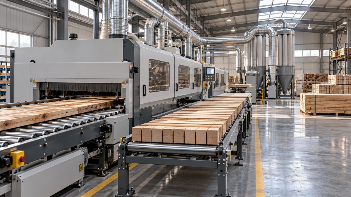
The system constraint matters more than the isolated machine rate. Faster rough cutting will not increase shipments if drying, moulding, assembly, or finishing remains the bottleneck. In that situation, the investment may still be justified by yield or labor savings, but additional sales contribution should remain outside the base case unless the downstream constraint is resolved.

Acceptance trials should therefore use representative stock and a realistic order mix. Record accepted output, timber consumption, total staffing, changeover time, and tooling usage—not merely the best continuous run.

A worked payback calculation

Consider a hypothetical investment of $200,000, including equipment, delivery, installation, training, initial spares, and additional working capital. The figures below illustrate the calculation; they are not market benchmarks or supplier performance claims.

Ignoring ramp-up, simple payback is $200,000 ÷ $65,000, or approximately 3.08 years. Suppose the first year produces only $32,000 of net benefit because utilization builds gradually. After three years, cumulative recovery is $162,000: $32,000 plus two years at $65,000. The remaining $38,000 takes approximately 0.58 years to recover, placing payback at about 3.6 years from the initial investment.

This simplified calculation assumes an upfront investment and evenly generated benefits within each year. An approval model should use actual payment milestones and expected monthly cash flows, particularly where deposits precede commissioning by several months.

Test the assumptions that can change the decision

A single payback estimate conceals the investment’s dependence on utilization, demand, yield, and staffing changes. Those assumptions should be varied together where they are connected. Lower production, for example, can reduce both material savings and additional sales contribution while leaving maintenance contracts largely unchanged.

These scenarios retain the same $200,000 investment and assume stable benefits after year one. They demonstrate how operating assumptions—not merely the purchase price—can move the recovery date.

Reverse the calculation to expose the approval threshold. If recovery is required within four years and first-year benefit is $32,000, the remaining three years must generate an average of $56,000 annually. That becomes a useful operating requirement against which to test the staffing plan, yield evidence, and supported order volume.

Removing speculative sales contribution is another revealing test. In the base example, excluding the $20,000 sales benefit reduces steady annual net benefit to $45,000. This identifies how much of the investment case depends on commercial growth rather than cost reduction.

Keep financing, tax, and ownership risk visible

Project economics and financing affordability answer different questions. An unlevered project model evaluates operating cash flows before financing and uses an appropriate discount rate. An equity cash-flow model includes loan proceeds and debt service. Mixing the two can double count financing costs or obscure the actual cash commitment.

Depreciation is not a cash outflow, although applicable tax treatment can affect after-tax returns. Use jurisdiction-specific tax assumptions consistently. A project that meets a simple payback target can still create a liquidity problem if debt repayments begin before production benefits stabilize.

Ownership risks also belong in the cash-flow assessment. Imported equipment can expose the buyer to exchange-rate movements, specialist travel costs, spare-parts lead times, and longer recovery from failures. Evaluate these through identifiable cost allowances and downtime scenarios rather than an unsupported contingency percentage.

Approval is strongest when the recovery date can be traced to evidence: installed-cost quotations, representative production trials, an achievable staffing change, supported demand, and a funded maintenance plan. If payback requires uninterrupted full-speed operation, immediate payroll reductions, and uncommitted sales simultaneously, the calculation describes an optimistic outcome rather than a reliable investment case.